I flock, you flock

by Vojtěch Tomas (@vojtatom), winter 2019/2020, exploring the flocking algorithm

The flocking algorithm mimics behaviors commonly seen in nature. A typical example of this behavior is the flight of birds in a flock. In this post, I'd like to go through the intricacies of the implementation both on CPU and GPU using compute shaders, and share some of the results I got. Inspired by The Coding Train Coding Challenge - Flocking Simulation by Daniel Shiffman .

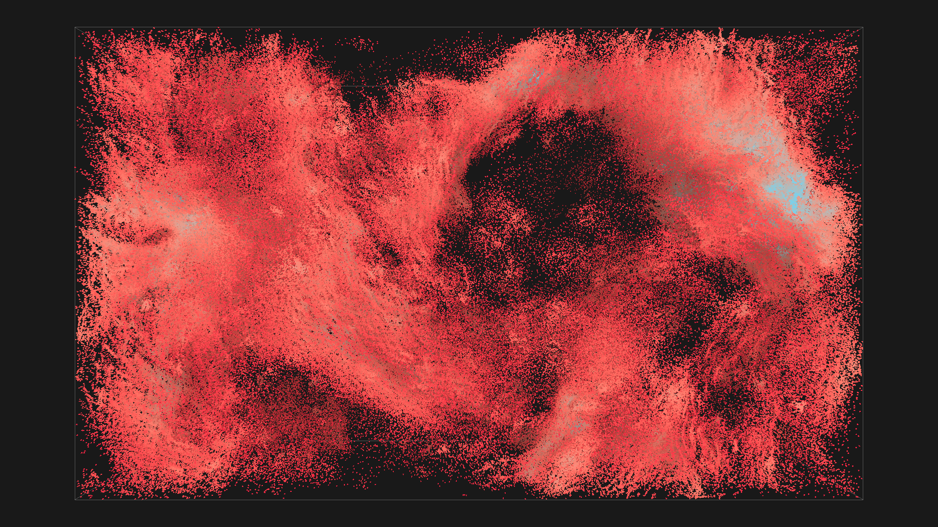
2^20 boids in red with depth shadowing, simulated using regular grid on GPU

So, what is the Flocking Algorithm?

The flocking algorithm was first presented in 1987 by Craig Reynolds [1, 2]. From the very beginning, the goal was to mimic behavior commonly seen in nature - the flight of birds in the sky or movement of fish in the sea. When we look at the algorithmic steering behaviors, we usually expect some kind of centralized guidance. Some of the older algorithms trying to simulate the flocking behavior relied on the centralized approach; however, the centralized approach increases the overall complexity, and, what is most significant, the simulation lacks natural appearance.

Contrary to the centralized approach, Raynold's flocking algorithm models the behavior of each agent individually. These agents representing the birds or fish are also commonly referred to as boids. To some extent, the system of boids can be understood as a particle system. The original paper goes further into the differences between boids and particles, but it isn't really that relevant here. The sketch bellow is just a 2D illustration.

Illustration of the flocking algorithm in 2D with additional mechanics. Each boid has a unique DNA describing its speed limit, moodiness, health etc. The color corresponds to the mood of the boid - orange means happy, blue means depressed and pink-ish white is neutral. Boids can become depressed when they are too far or too close to other boids, they become unhappy when they are hungry, and some of them have a "genetic" disposition to be happier than others. Created with p5.js

How does it work?

The minimal example boid consists of three vectors - position, velocity, and acceleration. Each boid looks around and adjusts its settings according to the boids within a specific range. The adjustments are made according to four basic rules. The original paper introduced only three of them and you can find the fourth one in [3, 4]. The final four rules are alignment, separation, cohesion, and clarity of view.

Rules of flocking, from left to right: alignment, separation, cohesion, and clarity of view

Alignment

The rule of alignment takes the directions of all boids within a particular range and computes the average direction. This new direction is represented as a force vector, which is applied to the current velocity of the boid.

Separation

The second rule, separation, steers the boid to avoid crowding local flockmates. The force vector is obtained as the sum of all inverse direction vectors between the local boids.

Cohesion

The third rule, cohesion, ensures the boids stay relatively close to each other by steering toward the average position of local flockmates.

Clarity of view

The last rule takes into account the view field and navigates the boid to keep its view field clear.

All four rules are depicted in the picture above. In the end, we can add all four forces together, and the result corresponds to the boid's current acceleration. It is also quite common to limit the amount of force by clamping the length of each force vector by some constant. On the other hand, it is possible to increase the amount of force applied during each iteration by a different factor.

It is quite interesting to realize how many configurable parts there are in the algorithm. There is the flocking radius, followed by the maximum amount of force and amplification factor. The size of the desired unobstructed view field can also be configurable.

Outputs

Before we dive deep into the design and implementation details, here are some of the outputs:

Screen capture of the simulation, please don't mind the compression, viewing in 1080p recommended

Circles

I found a very nice thing - with a very small change, you can force the boids to form circles! I haven't been able to find any mention of this in any literature, but you can do this just by changing the shape of the flocking area (flocking area meaning the area visible to each boid). The example bellow uses a half-hemisphere oriented in the positive z-direction.

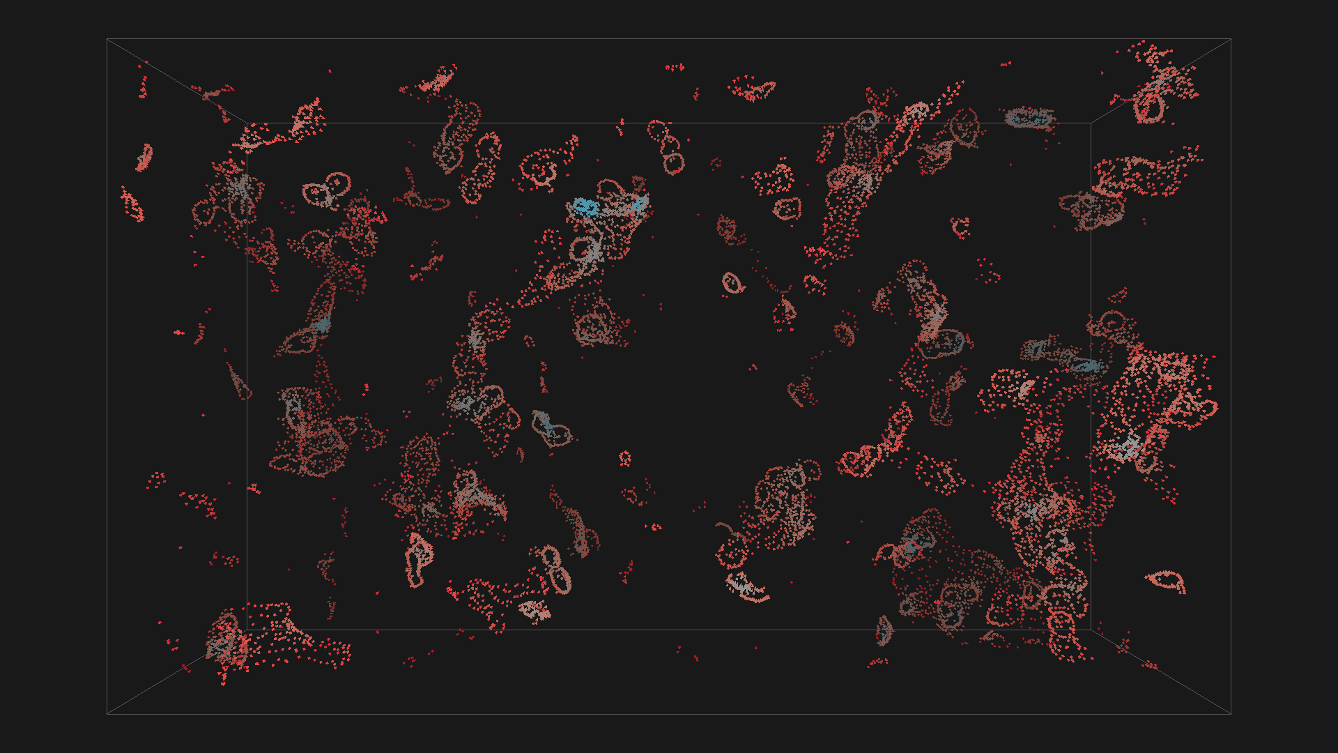
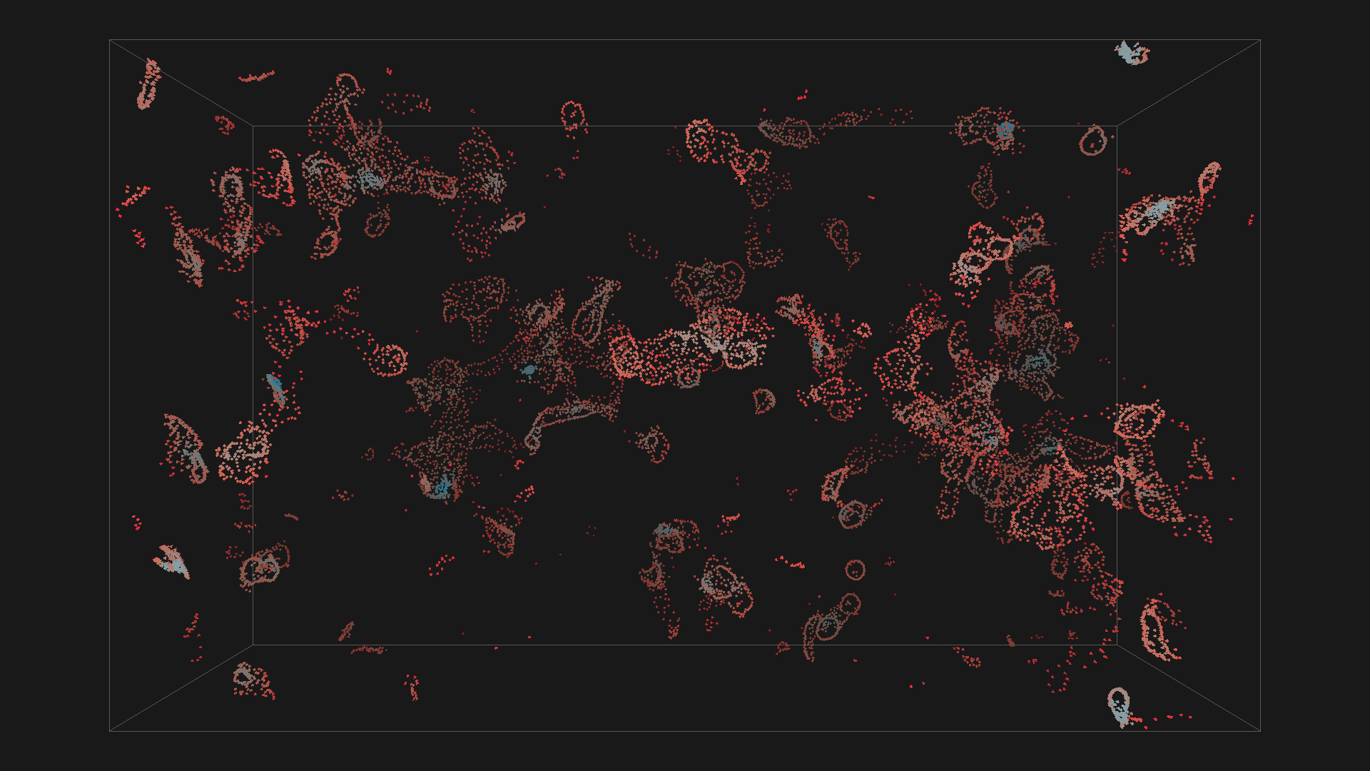
Boids forming circles, click for detail

The boids inside the aproximate half-hemisphere can be easily filtered using the grid-based approach, where you just ignore the boids inside cells "behind" the current boid. You can really start to see the circles around 0:20.

Boids forming circles

Design

The most straightforward approach would be:

                
for each boid as b:
    for each boid as e:
        if (e is in the flocking range of b) and (e is not b):
            accumulate forces from e to b
for each boid as b:
    apply accumulated forces to b
                
            

The obvious downfall of this approach is its quadratic complexity. The number of performed tests grows really fast, a single update of thousand boids requires millions of tests ( line 3 in the code above).

A better approach would be to parallelize the calculation (using CPU threads), but that would improve the performance only by a factor of thread count. In reality, only the closer boids have a higher chance of falling into the flocking range; therefore, most of the tests yield a negative result. An alternative approach - more relevant than a parallelization - is to organize the boids into a spatial data structure, e.g., octree.

Optimizing Flocking with Octree

The octree reduces the complexity of the algorithm close to n log(n), which is, to some extent, feasible. The pitfall of this approach is the necessity to reconstruct the structure each frame. It is possible to simply swap the data inside the tree; however, when the amount of changes reaches a critical limit, the tree becomes very unbalanced. It is just simpler to build the entire data structure from scratch.

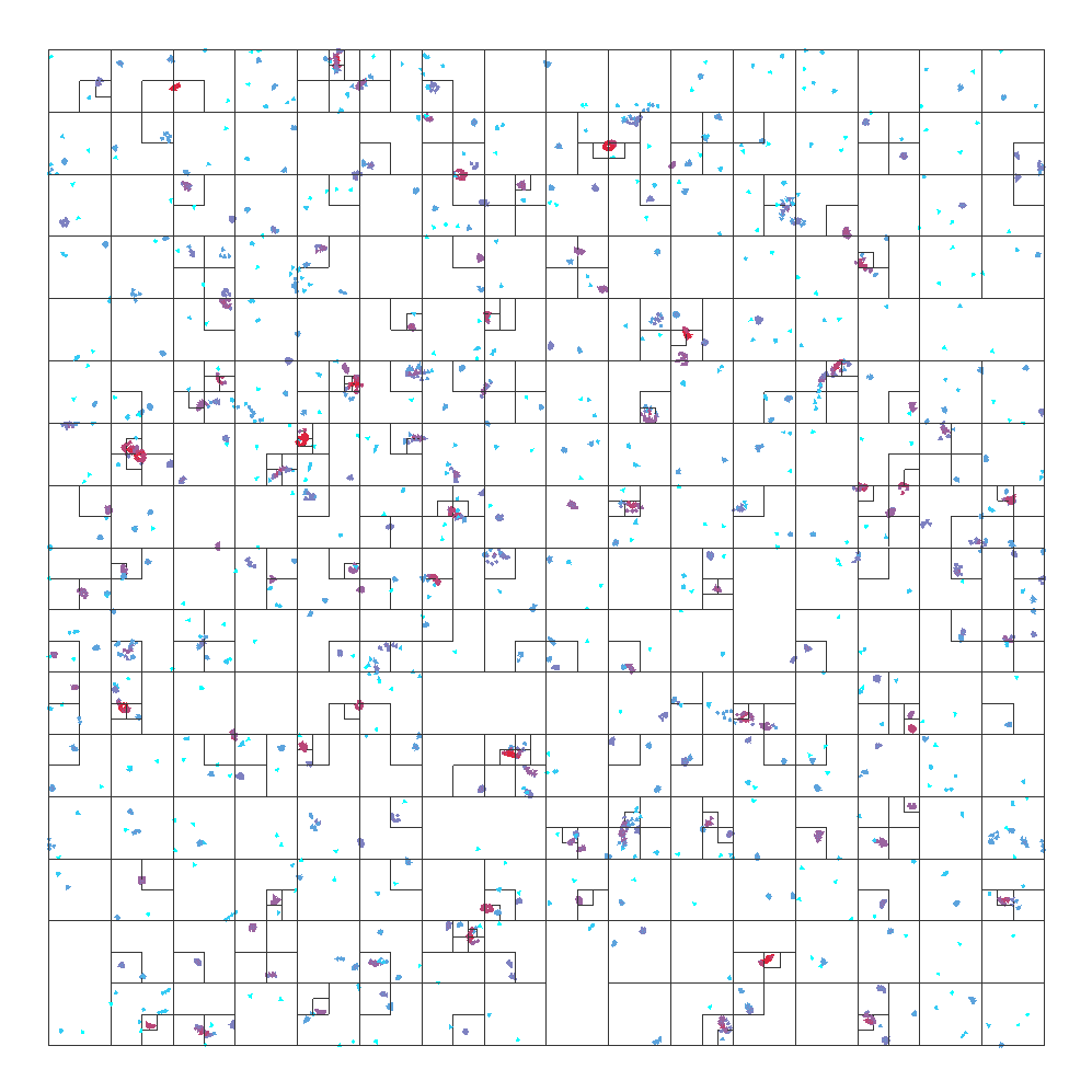
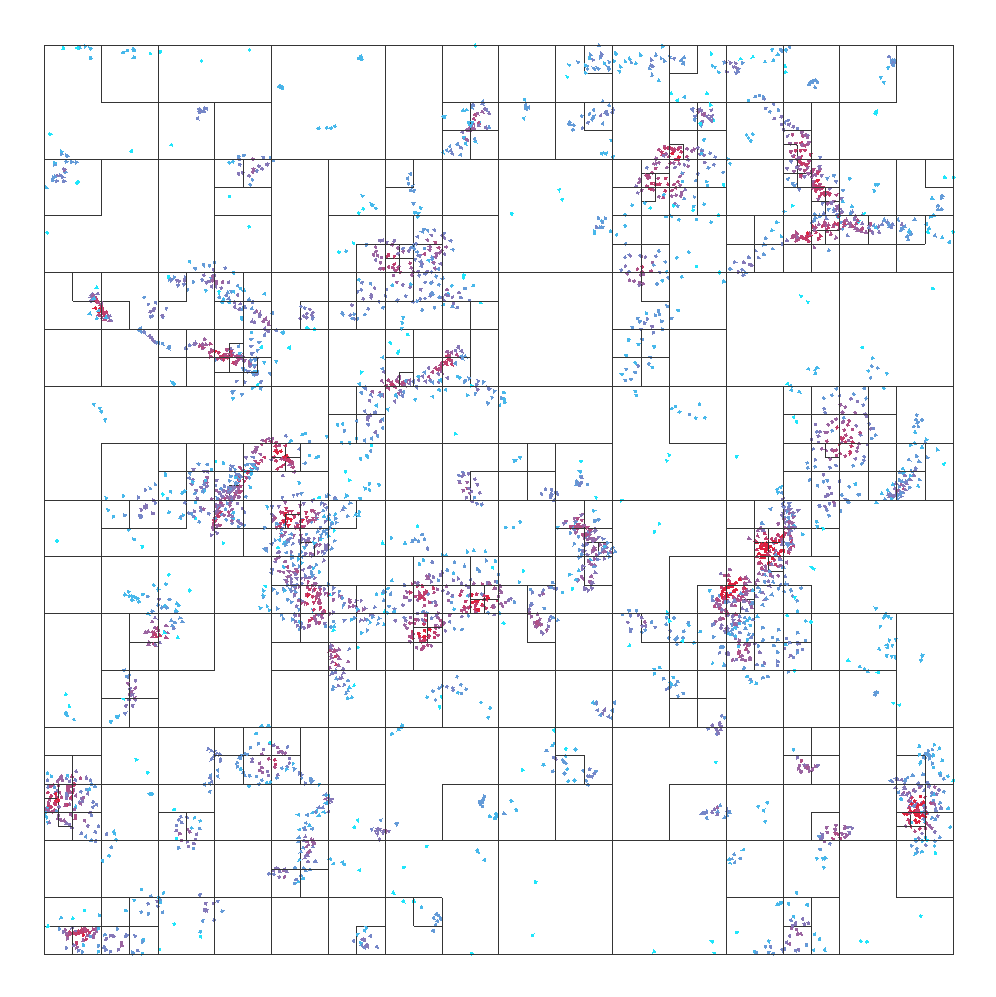
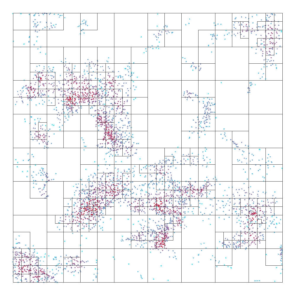
Impact of the different flocking algorithm settings on octree structure, from left to right the used flocking radius is 20, 40, and 60.

Nevertheless, since we really want to make the algorithm faster, n log(n) won't cut it, the main bottleneck is still the sheer amount of computations performed during the update. This is where the GPU comes into play.

Parallel Computation

To some extent, flocking could surely be listed as one of the embarrassingly parallel problems . If we had a computer that could run as many threads as the number of boids in parallel, each thread could calculate the acceleration of the assigned boid independently. But hold on, this can be effectively done using the GPU! Each GPU thread can simulate a single boid:

                
inside each thread:
    my_boid = boid[thread_id]
    for each boid as b:
        if (b is in the flocking range of my_boid) and (b is not my_boid):
            accumulate forces from b

sync all threads
    apply forces to my_boid
sync all threads
                
            

However, this approach solves only half of the problem. GPUs use SIMD or, more precisely, SIMT execution model , which allows for large amounts of data - boids in this case - to be processed in parallel.

The remaining issue here is the small number of boids which will fall into the flocking range. Checking all combinations of boids with a brute force approach can always be improved by organizing the boids into a spatial structure, enabling quick elimination of distant boids.

Grid-based Flocking

To further improve the efficiency of the algorithm, I considered two options:

• sorting according to a single axis projection,
• or organizing boids into a uniform 3D grid.

Both of these approaches are quite similar:

                
inside each thread:
    my_boid = boid[thread_id]
    my_boid.cell = compute which cell my_boid belongs to

sync all threads
parallel-sort the boids according to my_boid.cell
sync all threads

inside each thread:
    my_boid = boid[thread_id]
    for each "relevant cell" as c:

        #the boids in each cell can be accessed quickly
        #since the boids are sorted according to their current cell id

        for each boid in c as b:
            if (b is in the flocking range of my_boid) and (b is not my_boid):
                accumulate forces from b

    apply forces to my_boid
sync all threads
                
            

Alternatively, you can pick x, y, or z coordinate as my_boid.cell, the cells are going to represent long blocks spanning over the remaining dimensions. This approach always produces more candidates, which is visible in the image bellow. On the other hand, uniform grid takes into account all three spatial coordinates and will likely provide better results.

As mentioned earlier, the organization into a grid involves sorting the boids. To maximize the performance, the sorting should take place on the GPU as well.

If we use the 3D uniform grid, the flocking candidates are located inside the twenty-seven cells containing and surrounding the current boid (in 2D it's only nine). The size of the cell should be set up, so that the cell sides are half the size of the flocking radius. This ensures that the lookup for all positions within the local cell would return all of the boids within the range, provided we traverse the local and twenty-six surrounding cells.

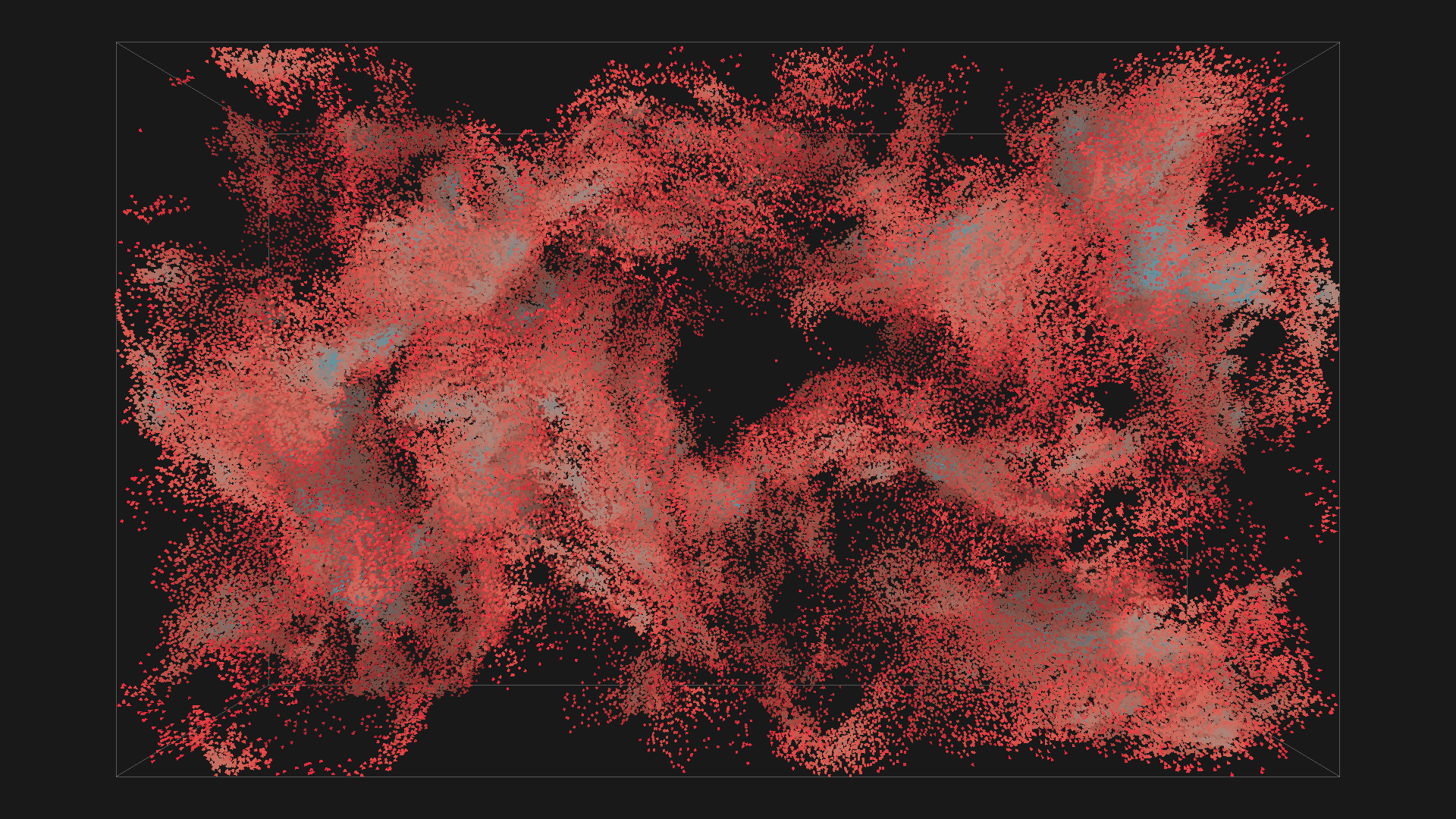
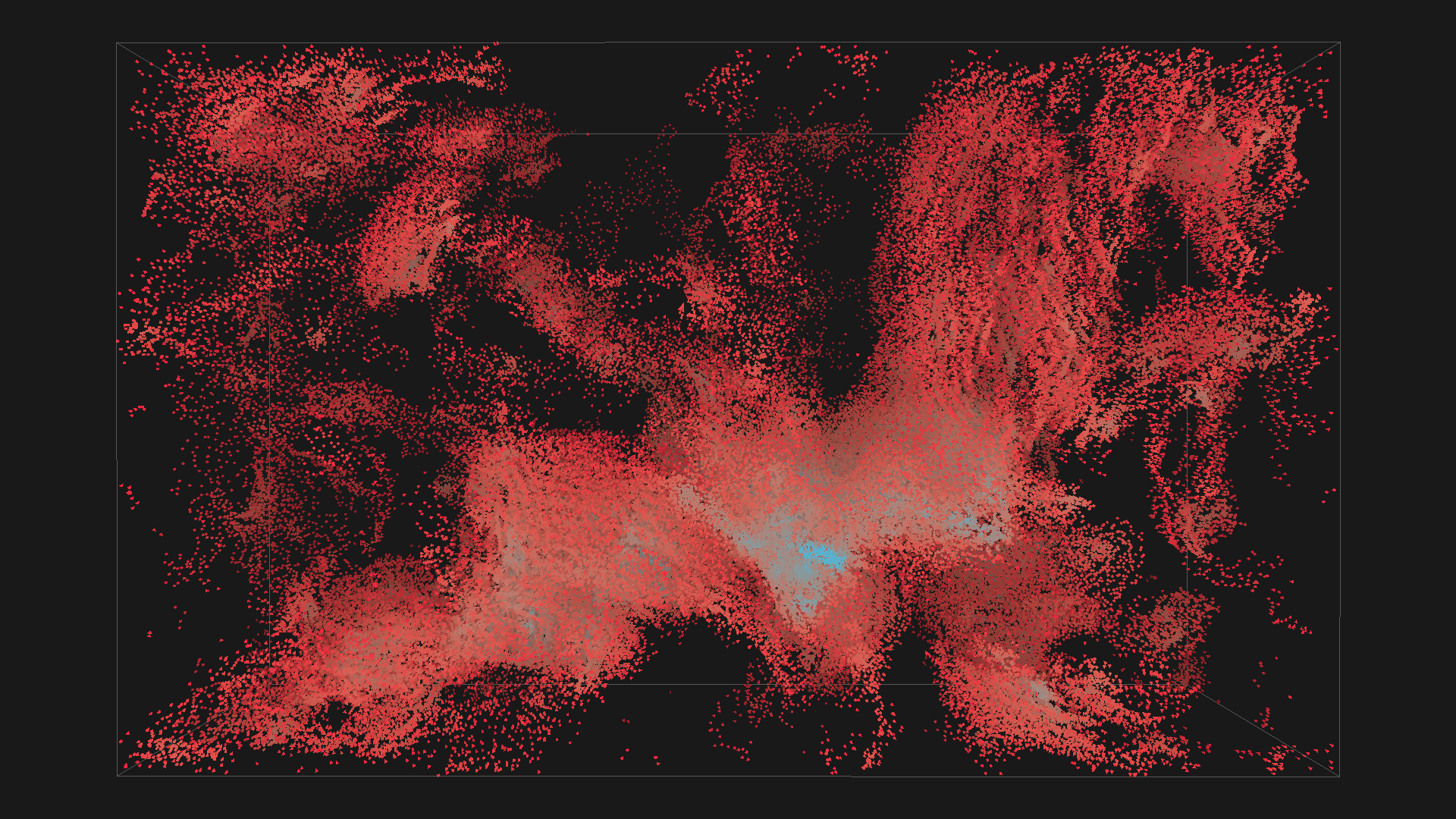
2^16 boids in red with depth shadowing

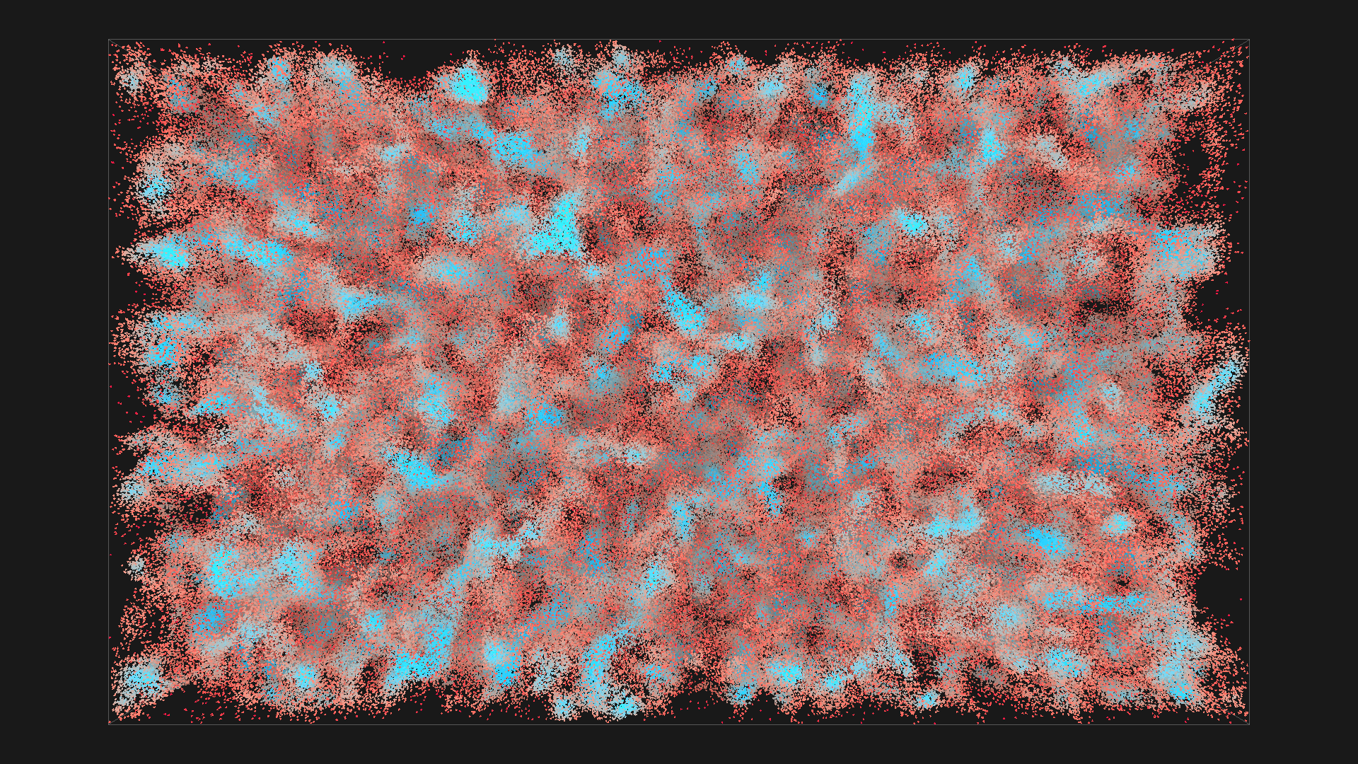
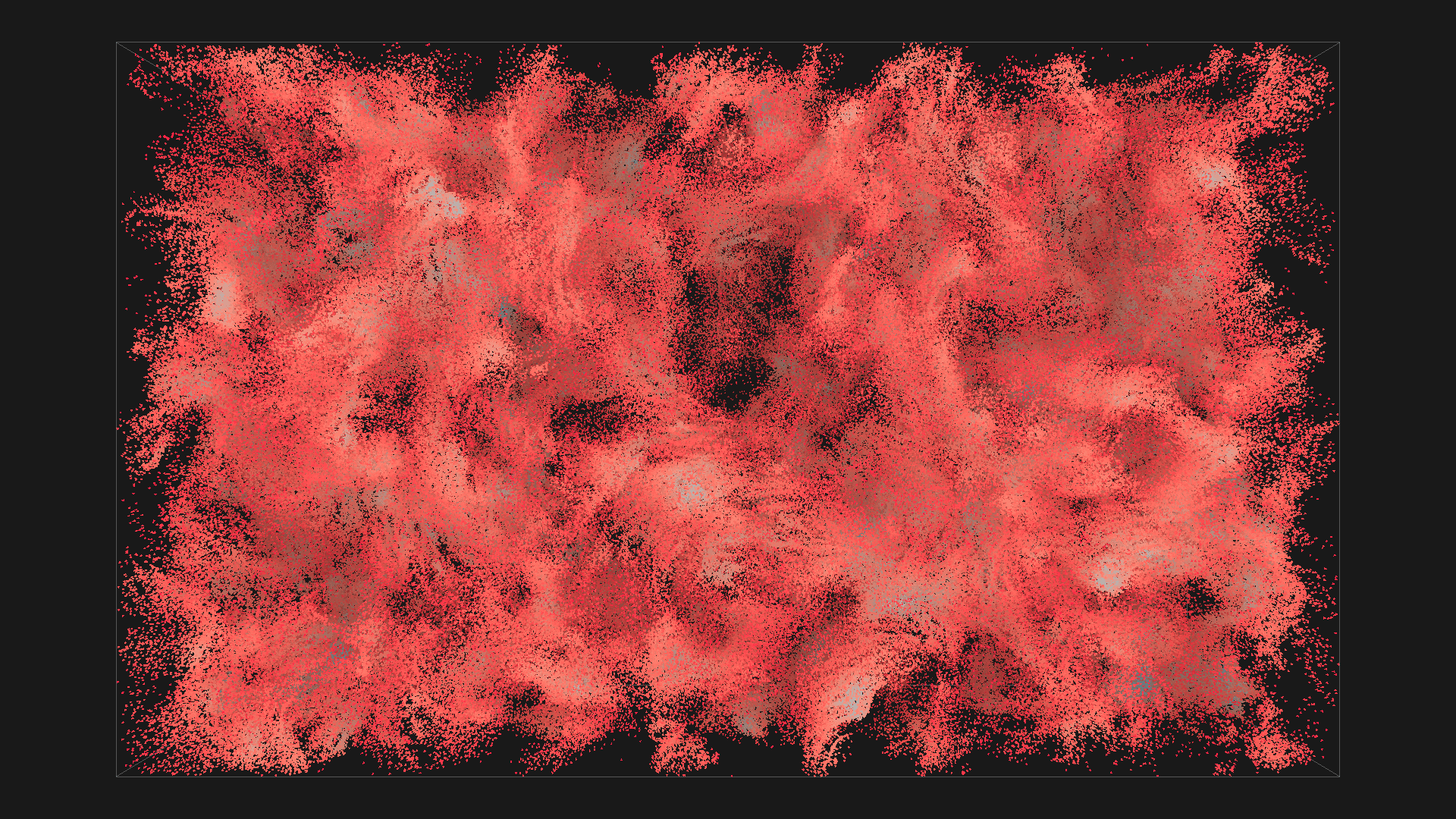
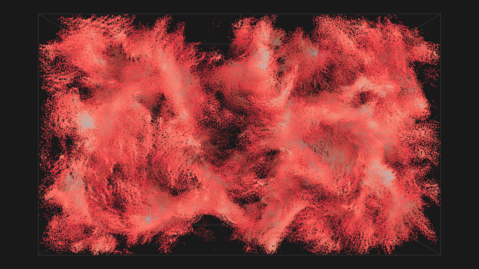
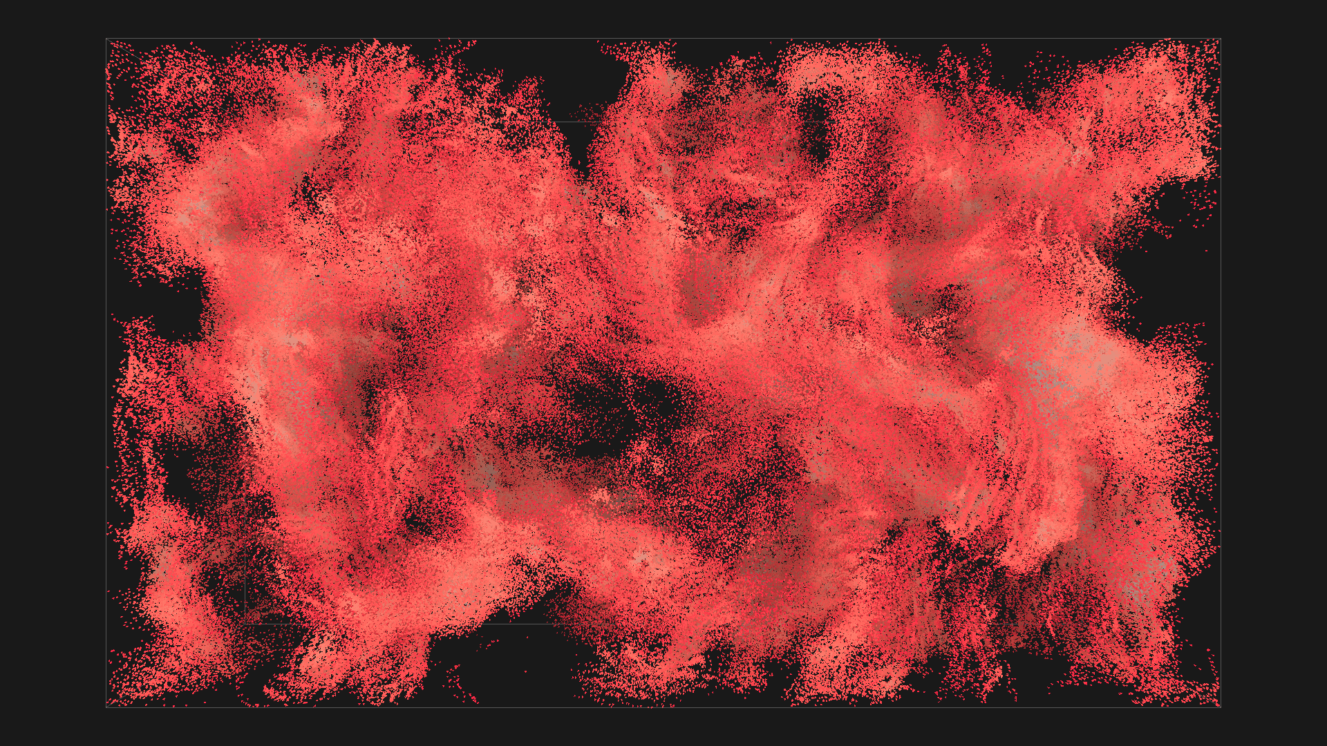
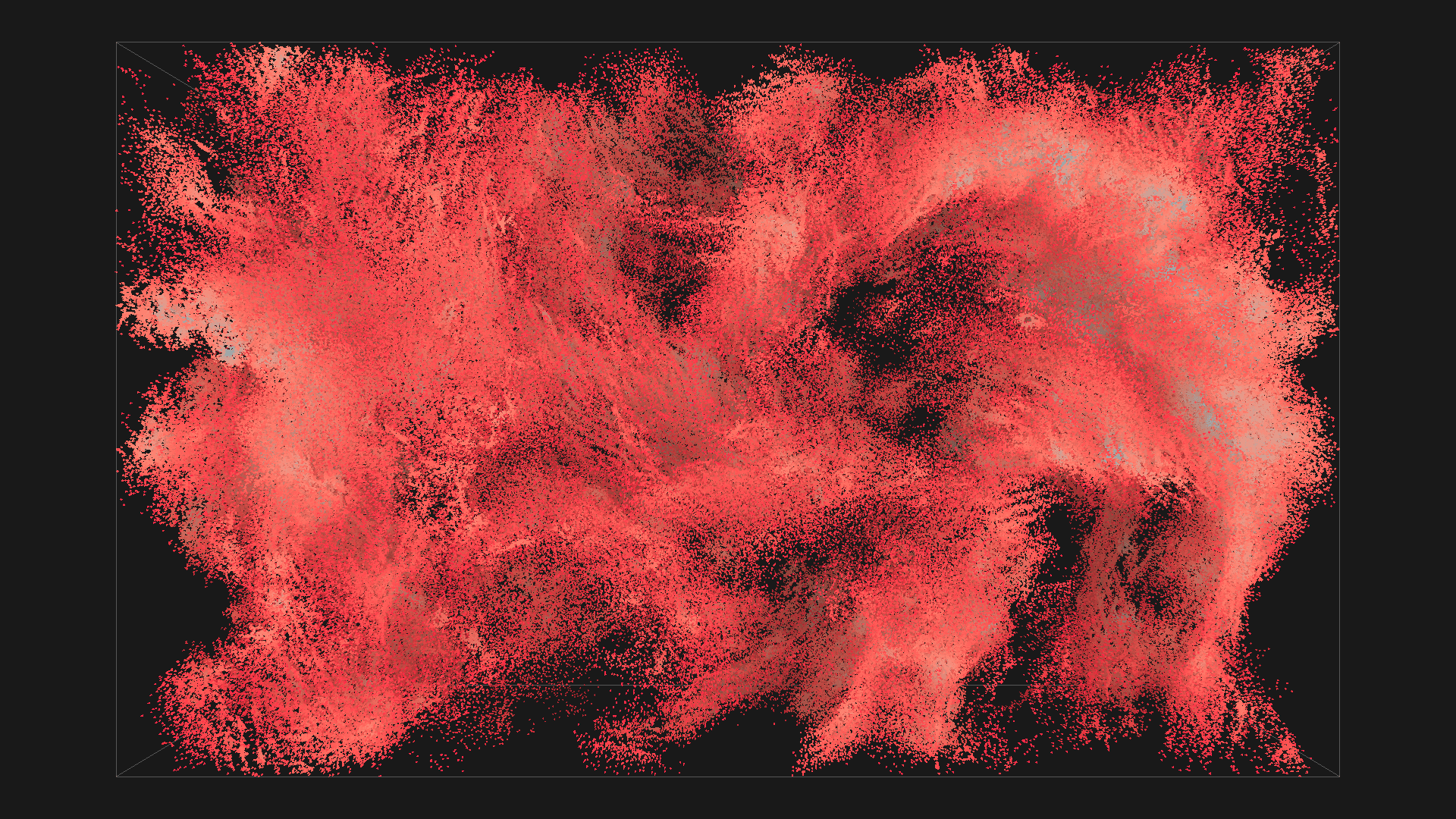
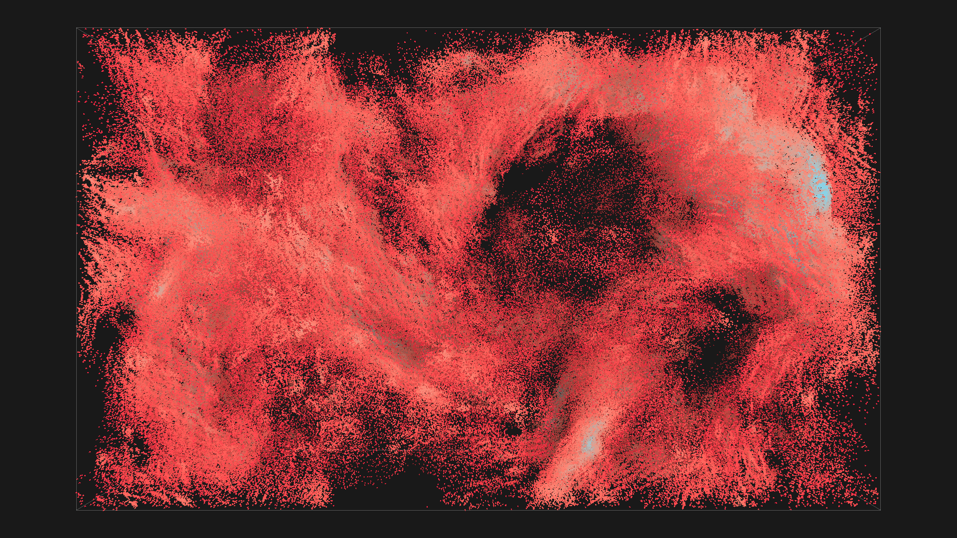
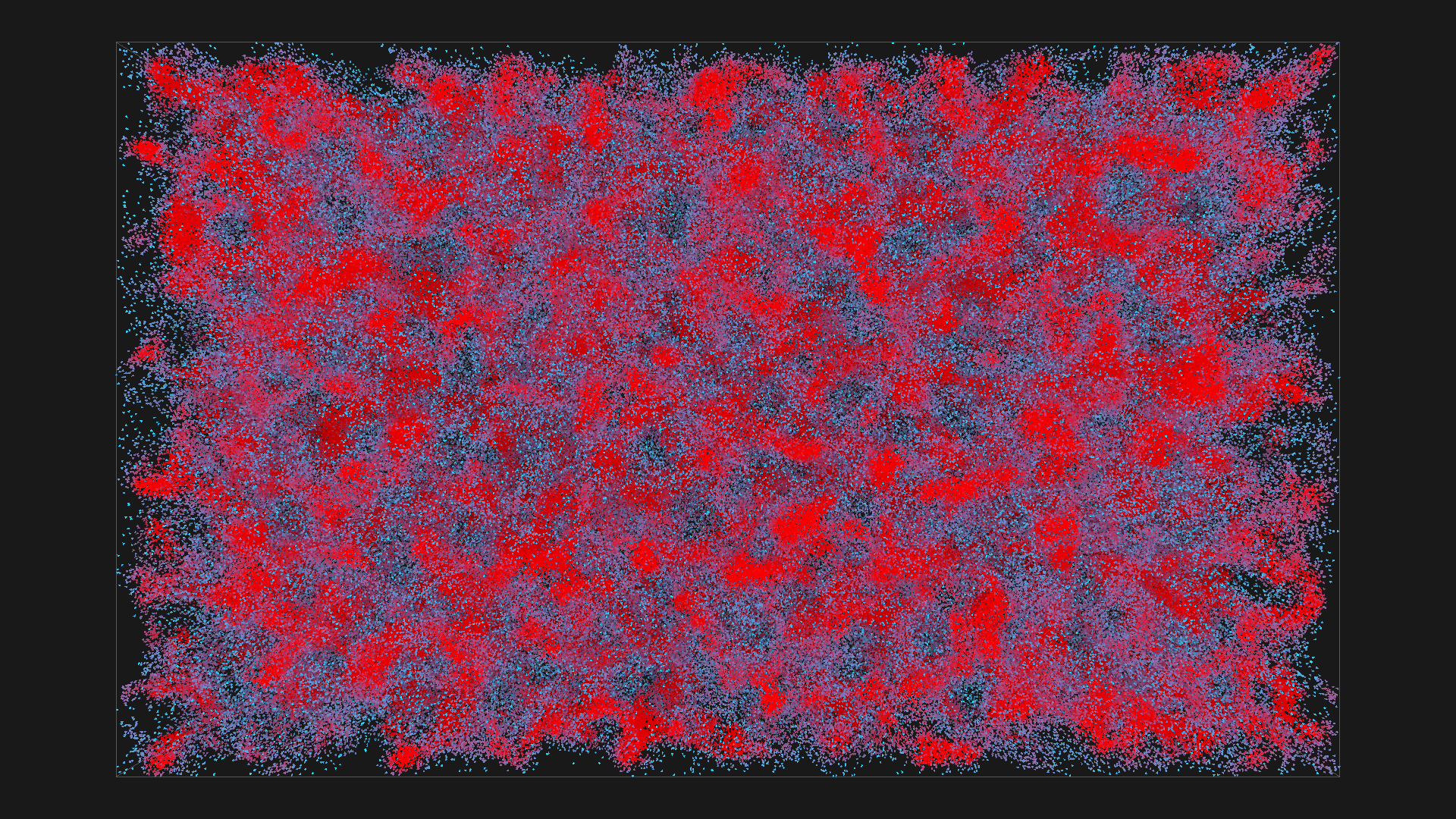
2^20 boids in red with depth shadowing, all images are from the same simulation, ordered chronologicaly

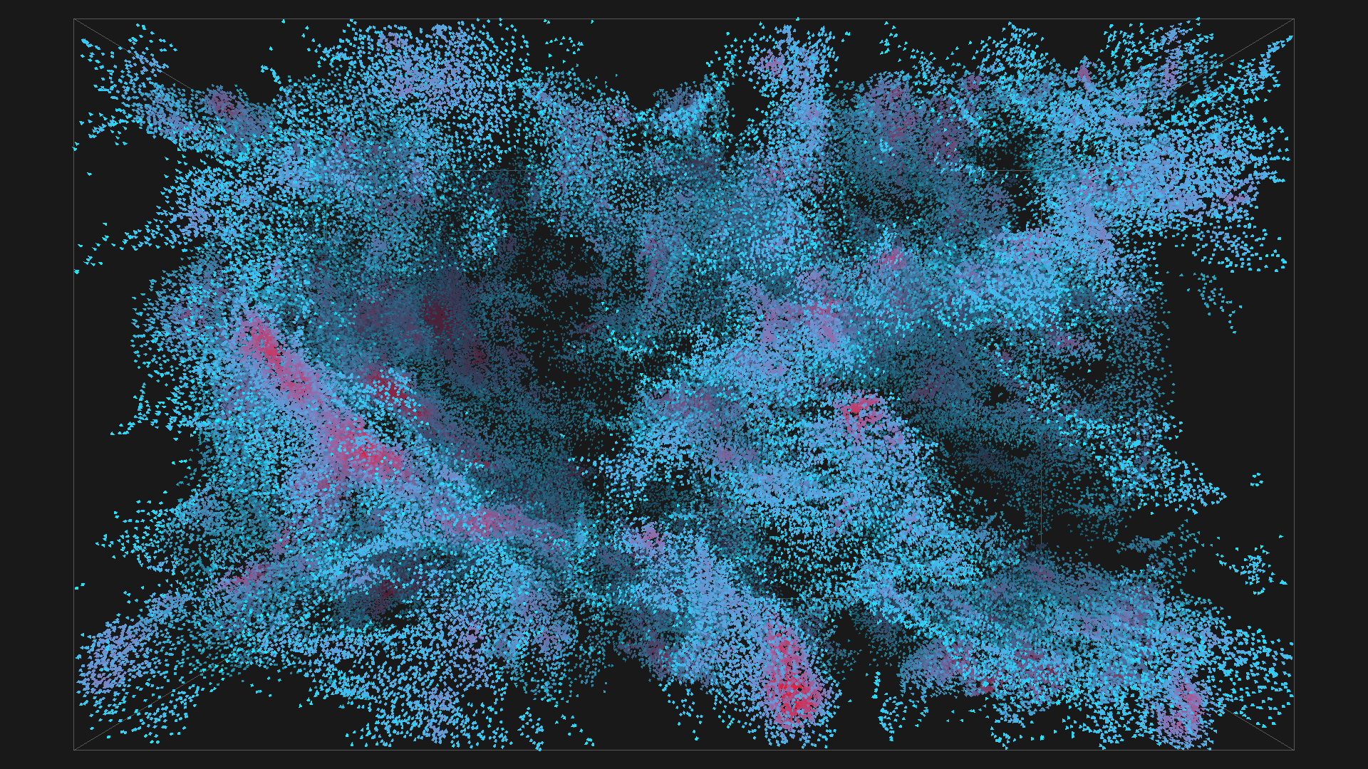
2^16 boids in red with depth shadowing

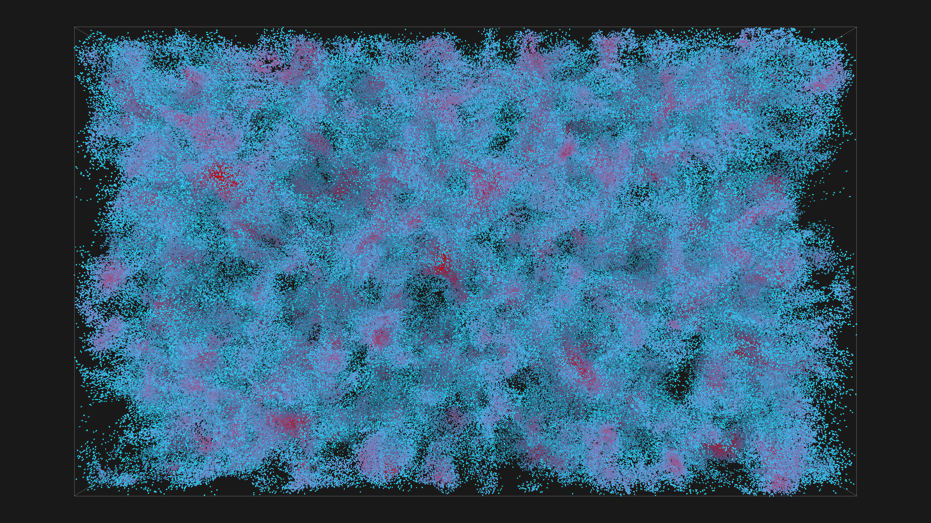
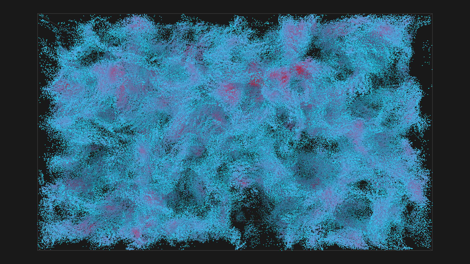
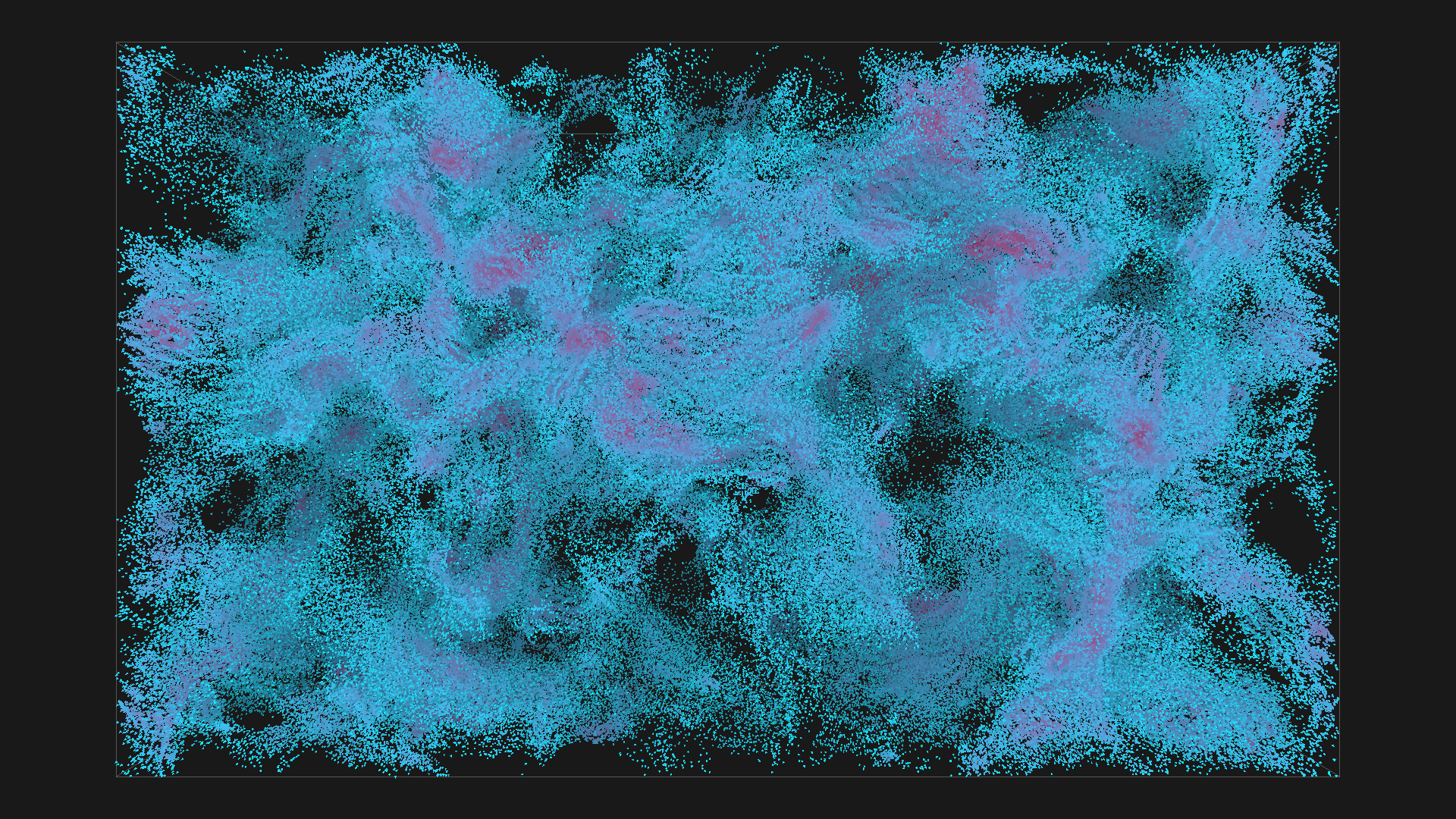
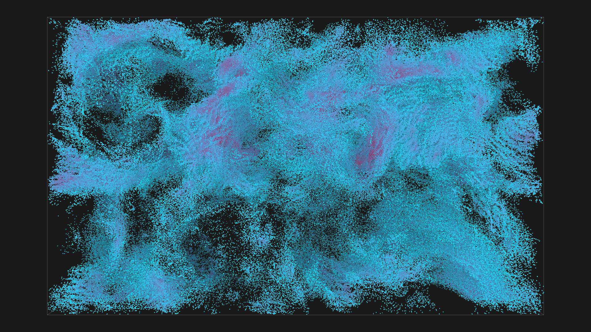
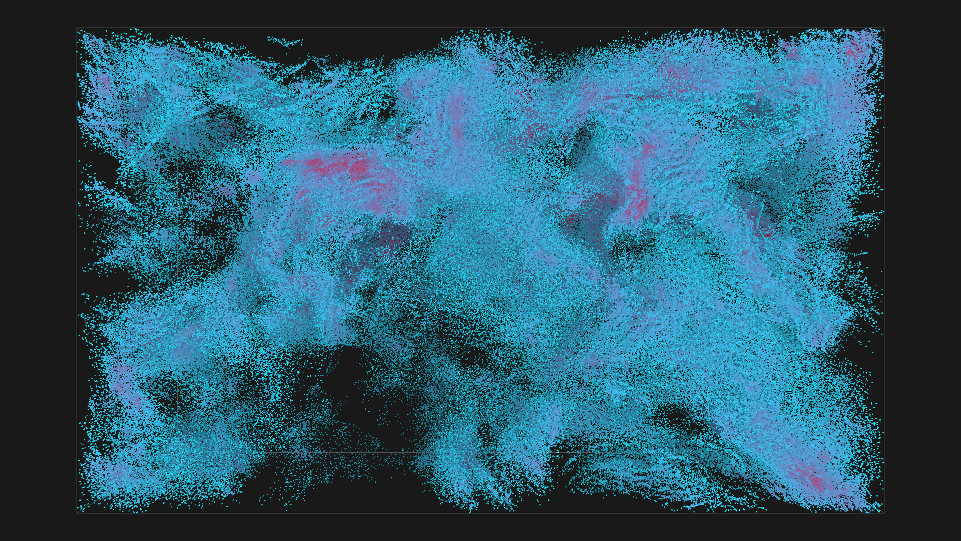
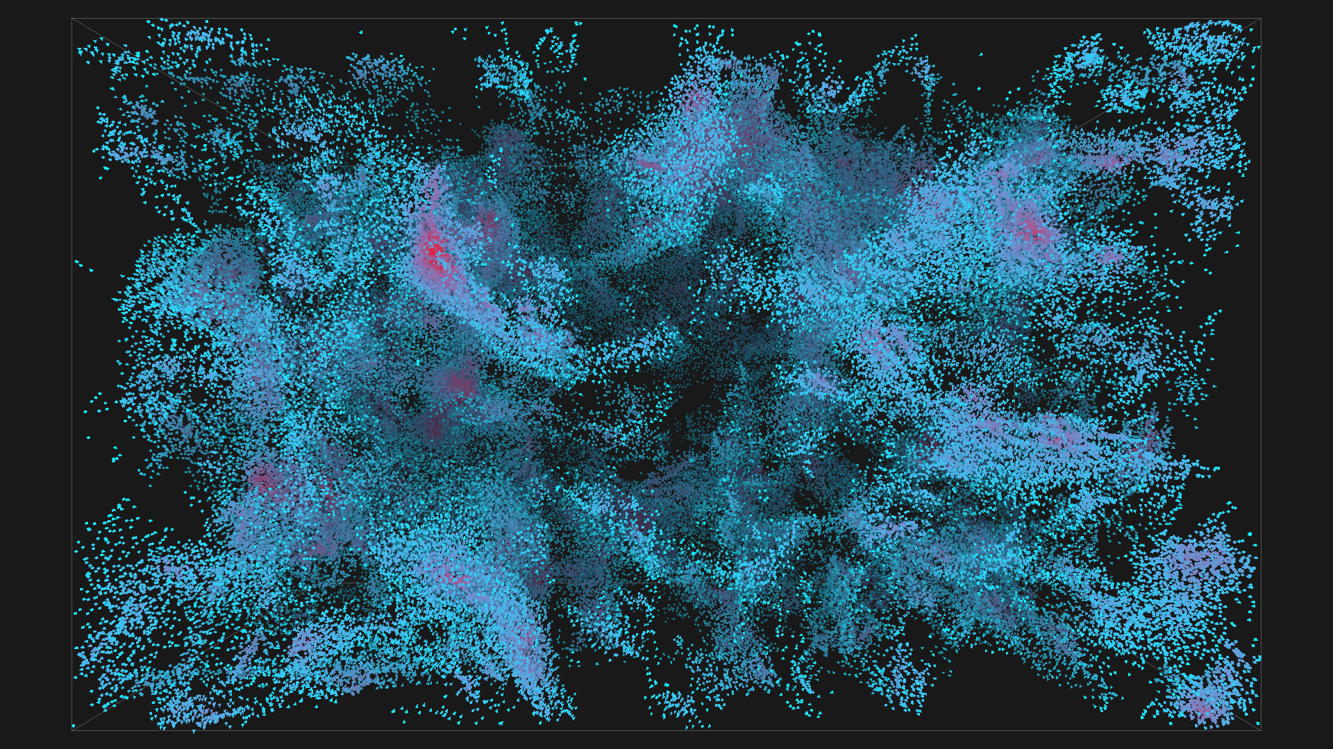
2^20 boids in blue with depth shadowing, all images are from the same simulation, ordered chronologicaly

Implementation

I decided to use OpenGL for drawing the boids and bounding boxes and OpenGL Compute shaders for the implementation of the parallel computations. I have tested all the mentioned approaches, except for the single-axis projection. That approach seemed similar to the one utilizing a grid, except less efficient, thus not worth implementing.

Bugs and Pitfalls

I got stuck several times during the implementation - however, the most significant pitfall regarded the memory alignment of data in compute shaders. When the data is transfered from the CPU to the GPU, the Bytes are copied as is and there is no padding involved. However, the internal type in GLSL vec3 - type useful for vector representation - is always 16-Bytes-aligned.

That means each two vec3 next to each other would have a 4-Byte padding between them. However, the data copied from the CPU is tightly packed, and to utilize these types in data layout specification requires manually padding each vector with any 4-Byte type.

There are two fixes available - to add the desired padding or to just simply work with float[3] arrays instead of vectors. The obvious choice would normally be the first approach. However, then I discovered this thread [5] , which mentions that the support for the manual padding is rather fuzzy, and the use of vector variables should be avoided. So, I went with float[3] instead.

What I actually made

I made an OpenGL app (github repo) . The app is configurable by changing the parameters in the environment file (see env.txt). Also, Doxygen documentation is attached to the project. There are four mutations of the implementation:

• CPU naive
• CPU octree-based
• GPU brute-force
• GPU regular grid

Each version is encapsulated in a single simulation engine class. The first two classes are pure CPU implementations of the flocking algorithm, and the last two utilize Compute shaders.

CPU naive and octree implementation

The naive CPU implementation is rather uninteresting, and it could be improved in so many ways, e.g., with the use of SSE instructions and threads. The enhanced CPU engine utilizes octree. An interesting detail about the octree is the implementation optimized for faster reconstruction.

Each frame, the tree is constructed from scratch. Therefore, it is necessary to avoid reallocation of the tree nodes at all costs. Each tree node is supposed to have eight child nodes; however, some of those nodes could easily stay uninhabited. There is no point in even constructing such nodes. The tree works with a buffer of reusable nodes, and all used values are tightly packed.

GPU brute-force implementation

The naive GPU implementation processes one boid per invocation. Each invocation picks a boid and then linearly iterates through all other boids. The nice thing about this approach is its simplicity; there is no sorting involved. The unfortunate thing is the need to read from global memory. It would be possible to copy a chunk of boids from the global memory into the local shared memory first; however, that has been left as a possible improvement for future version.

The main advantage of the naive GPU implementation can be demonstrated when compared with the CPU octree implementation with high densities of boids in isolated locations. These centers cause the tree range queries to stall. The performance of the octree in this situation is almost equivalent to the performance of the naive CPU implementation with the added cost of tree traversal. The naive GPU implementation can eliminate the cost of sequentially repeated range search for each boid.

GPU grid-based implementation

The core idea behind this version is to combine the speedups gained by parallelization while providing a faster way to perform range queries by sorting the data according to a particular grid.

One technical detial worth mentioning is the implementation of the bitonic merge sort. The implementation is designed to utilize all dispatched invocations and to maximize the benefit of using shared memory inside the local workgroup (and also minimize the number of global sync points) (basically it's cool). Look at the source code for more info.

Benchmarks

Out of curiosity I tested the implementation on two computers; the goal was to measure the computation time of a single frame. According to expectation, the GPU implementation beat the sequential CPU implementation by orders of magnitude. It was not possible to measure some data samples on both GPU and CPU purely because of the CPU implementation performance.

Config A: Linux Kubuntu 18.04, Intel Core i7 7700 @ 3.6GHz, RAM 8GB DDR4 2133MHz, NVIDIA GeForce GTX 1060 6GT

Config B: Windows 7 SP1, Intel Core i5 3335S @ 2.7GHz, RAM 8GB DDR3 1600MHz, NVIDIA GeForce GT 640M

The benchmark used diferent sizes of the flocking area (box size is noted in the graphs, it is scaled according to the number of boids). Used parameters are flocking radius 20, force limit 0.1, and speed limit 2.0. The CPU octree and GPU grid-based versions are density-sensitive, meaning that the speed of execution is also limited by the spatial density of the boids.

Conclusion

Feel free to look at the code, experiment with it, mail me or tweet @vojtatom (me) if you decide to make something based on this.

1. REYNOLDS, Craig W. Flocks, herds and schools: A distributed behavioral model. ACM, 1987.
2. REYNOLDS, CRAIG, 2001, Boids (Flocks, Herds, and Schools: a Distributed BehavioralModel). Red3d.com [online]. 2001. [Accessed 13 January 2020]. Available from link
3. SHIFFMAN, Daniel; FRY, Shannon; MARSH, Zannah. The nature of code. D. Shiffman, 2012.
4. FLAKE, Gary William. The computational beauty of nature: Computer explorations of fractals, chaos, complex systems, and adaptation. MIT press, 1998.
5. BOLAS, NICOL, 2016, Should I ever use a ‘vec3‘ inside of a uniform buffer or shader storage buffer object?. Stack Overflow [online]. 2016. [Accessed 13 January 2020]. Available from link